Data Structures and Big O For Coding Interviews - Data Structures Explained
Data structures click when you pair them with Big O notation, because that shows how fast operations like access, insert, and delete scale as your data grows. Constant time O(1) is instant, linear O(n) grows with your data, logarithmic O(log n) speeds things up by halving the search each step, and quadratic O(n^2) explodes when every item touches every other. Arrays, linked lists, stacks, queues, heaps, hashmaps, binary search trees, and sets each shine in different scenarios based on those costs. Pick the one that matches your pattern, and your code feels like flying instead of walking.
Hey, I’m Sajad. I’ve got a bachelor’s and a master’s in computer science from Georgia Tech, spent time building software at places like Amazon, and every single day I help hundreds of thousands of people break into tech.
This piece is me taking a beat to write down what I teach in videos - the core data structures, how they work, where they fit in real life, and the Big O time costs that matter in interviews.
You’ll see pictures in your head - lockers, trains, chip stacks, store lines, box pyramids, mail rooms, family trees, and yes, Thanos’s gauntlet - because when you can visualize it, you can explain it under pressure.
What Big O Really Means For Data Structures
Think of Big O like miles per hour, but for code. It’s how we measure the speed and efficiency of operations based on how much data we’re handling.
If I need to get from New York to California, I could walk, bike, drive, or fly. Each option is a different time cost for the same goal. Same thing with data structures - different structures get you to the answer with different time costs.
O(1) - Constant Time
This is the rocket ship. Super fast. The operation takes the same amount of time no matter how much data there is.
Picture a grocery list. If your task is “grab the first item,” it doesn’t matter if the list has 5 items or 5,000. You go to index 0 and you’re done. That’s O(1) - predictable and instant.
O(n) - Linear Time
This is the supercar. Still fast, but tied to the amount of data.
If you have a list of names and you’re looking for a specific one without knowing the position, worst case you check every single name. 10 names means up to 10 checks. 1,000 names means up to 1,000 checks. As the data grows, the time grows at the same rate.
O(n^2) - Quadratic Time
This is like biking across the country. Painfully slow as the data grows.
Imagine a class where everyone has to shake hands with everyone. If there are 10 students, that’s roughly 100 handshakes. If there are 100 students, that’s about 10,000 handshakes. Every item interacts with every other item - it balloons fast.
O(log n) - Logarithmic Time
This one is sneaky fast - like the speed of sound. Faster than linear, slower than constant, but wildly efficient at scale.
Think of a dictionary. You don’t go page by page. You open roughly in the middle, decide if your word comes before or after, then jump again. Each jump halves your search space. Half, then half of that, then half again. That shrinking search space is what gives you O(log n).
Arrays and Linked Lists - The Core Linear Structures
These are your bread and butter. They both hold sequences of values, but the way they store and move data is totally different.
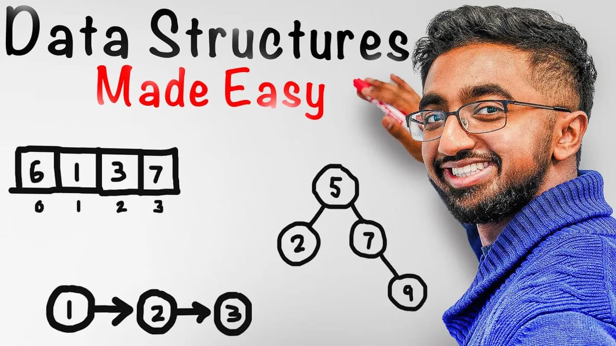
Arrays - Think Middle School Lockers
Picture a long row of lockers. Each locker has a fixed position. If someone says “locker 12,” you can walk right to it without peeking inside every other locker on the way.
That’s an array. Data is stored contiguously - side by side in memory - with each value sitting at a specific index.
Access by index is O(1) because you can jump straight there. No searching, no wandering.
But there’s a catch. Arrays are fixed in size. If the array is full and you want to add another value, you can’t just squeeze it in. You create a new larger array and copy everything over, then add the new item.
That resizing step is O(n) because of the copying. Replacing an existing element by index is O(1). Deleting from the end is O(1). Deleting anywhere else is O(n) because the remaining elements must shift to stay contiguous.
And yes, there’s a structure similar to an array that handles resizing better. If you know which one I’m hinting at and why it’s better, drop it in the comments. I might shout you out next time.
Linked Lists - Think Trains, Car By Car
Now imagine a train. Each car is connected to the next one. If you want the 8th car, you start at the front and walk back car by car until you reach it.
That’s a linked list. Each node holds a value and a pointer to the next node. Sometimes there’s also a pointer to the previous node in a doubly linked list.
Access by index is O(n) because there’s no instant jump - you traverse. But insertion and deletion can be O(1) if you already have a reference to the node you’re inserting around or removing. No shifting, no copying - just rewire the pointers.
If you don’t have the reference and you need to search for it, the traversal makes it O(n). The upside is there’s no resizing stress like arrays. You’re just dealing with nodes and pointers.
Stacks and Queues - LIFO vs FIFO In Real Life
Stacks and queues are simple but powerful. One is last in, first out. The other is first in, first out. You use them constantly in algorithms.
Stacks - The Chip Stack On Game Night
Imagine a stack of chips. You eat the top one first. To get to the chip below, you first remove the top. That’s LIFO - last in, first out.
With a stack, you can push to the top and pop from the top. That’s it. No browsing through the middle. No skipping ahead.
Push is O(1). Pop is O(1). If you do need to search or access an element deeper down, you’re effectively peeling off items one by one, so worst case that’s O(n).
Stacks are used everywhere in depth first search, undo operations, call stacks, balanced parentheses problems, and more. The simplicity is the whole point - it makes adding and removing lightning fast.
Queues - The Checkout Line At The Store
Think of a line at the grocery store. The first person in line gets served first. Anyone new joins at the back and waits their turn. That’s FIFO - first in, first out.
Queues insert at the back and remove from the front. You don’t cut in the middle. You don’t grab from the center.
Enqueue is O(1). Dequeue is O(1). If you attempt to search for an element inside, that’s O(n) because you’d scan through.
Queues are the backbone of breadth first search and, fun example, they literally power your Spotify queue - songs get added at the end and played from the front in order.
Heaps (Priority Queues) - Always Grab The Top
Now picture a pyramid of boxes. The smallest box sits at the very top. You always take from the top. If you remove a box somewhere else, everything readjusts so there’s still a valid top box.
That’s a heap. Two flavors you should know: min heap and max heap. In a min heap, every parent is smaller than its children, so the smallest element lives at the root. In a max heap, every parent is larger than its children, so the largest element is at the root.
Heaps are complete binary trees under the hood. The structure enforces “parent before children” ordering, not full sorting. You get quick access to the top priority element and efficient insertions and removals.
Peek at the top is O(1). Insert is O(log n) because you place the item and let it bubble up to its correct spot. Remove the top is O(log n) because you pop the root, move the last element to the top, and bubble it down to restore the heap property.
Accessing an arbitrary element inside a heap isn’t a typical operation. If you truly need to find a random element, that’s O(n) because heaps don’t store elements in a way that supports fast searches beyond the root.
Hashmaps, Binary Search Trees, and Sets - Fast Lookups Three Ways
These three all help you find things quickly, but they go about it in different ways. One hashes keys, one orders values in a tree, and one enforces uniqueness.
Hashmaps - The Office Mailroom
Imagine a mailroom with labeled mailboxes. John’s mailbox is 4. Sally’s is 5. You don’t sort through every envelope - you go straight to the right box.
That’s a hashmap. You store data as key-value pairs. The key runs through a hash function that maps it to a slot in an array-like structure. If we use a playful example hash function - the length of the name - John maps to 4, Sally maps to 5.
Lookups by key are O(1) on average because hashing gives you the slot instantly. Inserts and deletes are also O(1) on average.
But collisions happen. If Andy shows up and his name also hashes to 4, John and Andy can’t both live in the same exact slot. We fix that with collision resolution - either by chaining (a linked list from that slot) or by probing (scan for the next available slot).
Worst case, if collisions go wild and everything piles up in a chain, lookups, inserts, and deletes can degrade to O(n). With a solid hash function and good load factor management, you usually stay in O(1) land.
By the way, in Python you probably call hashmaps dictionaries. Same idea, slightly different name.
Binary Search Trees - The Structured Family Tree
Picture a family tree, but with a rule. Every node has up to two children. The left child’s value is smaller than the parent. The right child’s value is larger.
That rule lets you drive your search like the dictionary trick. If the value you want is smaller than the current node, go left. If it’s larger, go right. Each step tosses out half the remaining values.
When the tree is balanced, access, insert, and delete are O(log n). That’s the logarithmic search magic - cut the space in half, again and again.
Worst case, if the tree becomes unbalanced and leans into a line that looks like a linked list, those operations drop to O(n), because you might be walking node by node without that halving trick.
Sets - Thanos’s Gauntlet Of Unique Elements
Think of Thanos’s infinity gauntlet. Each stone is powerful and unique. Try to add the same stone twice - nope. The gauntlet refuses duplicates. The order doesn’t matter. What matters is whether the stone exists.
That’s a set - an unordered collection of unique values. Under the hood it’s often powered by a hash table, which is why checking for existence is O(1) on average, same for insert and delete.
Collisions can push those operations to O(n) in the worst case, just like hashmaps, but with a good hash function you stay fast.
Sets are perfect for keeping track of visited nodes in graph or tree traversals, removing duplicates from a dataset, membership checks, and classic set ops like union, intersection, and difference.
How To Practice This Stuff And Use It In Interviews
You’ve got the toolbox - now it’s about reps. The fastest way to make this second nature is to practice data structure specific problems that mirror what companies actually ask.
I put together a newsletter where I send out targeted LeetCode problems by company and by data structure. If you want to apply arrays, linked lists, stacks, queues, heaps, hashmaps, BSTs, and sets to the exact patterns you’ll see at places like Amazon or Google, you’ll like what I send.
It’s not about grinding everything. It’s about learning to recognize patterns. When you train your brain to map problem patterns to the right structure, you move faster and answer with confidence.
- Arrays - use when you need random access and tight memory layout
- Linked lists - use when inserts and deletes happen in the middle
- Stacks - LIFO logic like DFS, backtracking, and undo
- Queues - FIFO logic like BFS and task scheduling
- Heaps - always grab the min or max fast
- Hashmaps - constant time lookups by key
- BSTs - ordered data with near logarithmic operations when balanced
- Sets - fast existence checks and unique collections
Closing Thoughts
Data structures aren’t trivia. They’re your vehicles. Sometimes you need to fly. Sometimes you just need a solid drive. Big O tells you how fast each vehicle goes as the road gets longer.
Arrays, linked lists, stacks, queues, heaps, hashmaps, binary search trees, and sets each bring something specific. Use the right one and your solution feels simple. Use the wrong one and it feels like you’re walking to California.
If this breakdown helped, give it a like and subscribe so more learners find it. And if you’re aiming for a software engineering internship in summer 2025, I recorded a full video you can watch next - it’s packed with steps that work.